

A fanciful depiction of how a grid cell based navigation system could compute a direct path across unvisited regions of space.
A week ago Stensola et al published evidence that Entorhinal Grid Cells are modular, and on the same day I wrote a glowing commentary, The Significance of the Modular Organization of Grid Cells. In addition to praising the paper, I tried to explain why evidence for modular organization was welcome news, in that it supported computational mechanisms that grid cells could perform. In the rest of this post I outline a model Andre Fenton and I have been working on that relies on discrete modules of grid cells. Our model extracts a function we call linear look-ahead and uses this function for efficient navigation. We feel it represents the begining of a process of explaining high order cognitive functions at the neuron network level
Forewarning. This post is a bit esoteric. It’s aimed, primarily, at a hippocampal/entorhinal audience. In the post I’ll describe a process we call linear look ahead. I will describe how this could be implemented with a class of entorhinal neurons called conjunctive cells. I will describe how linear look ahead could be implemented in a single module. Finally, I will describe how linear look-ahead across modules could be used to find linear paths from an animal’s current location to a goal.
Linear Look-ahead is the computation I will describe. In linear look-ahead an animal sits at one location, point its nose in a particular direction and ‘computes’ the set of locations it would visit if i were to walk, in a straight line, in the direction of of its nose. Using linear look-ahead a animal can compute the shortest path between its current location and a goal. The constraint is that the animal must have taken some be familiar with a continuous ground surface that contains the current location and goal. But, most importantly, the animal does not have to be able to see the goal, and the computed path can cross unvisited space. The path, because it is linear, must be the shortest route between current location and goal.

Idealized conjunctive cell. Conjunctive cells fire in a grid pattern, but only when nose i pointed in preferred direction.
Conjunctive Cells are a second class of neurons in entorhinal cortex (Sargolini et al). Conjunctive cells have the bump-like properties of grid cells, but additionally are highly directional. That is, a conjunctive cell will fire if the rat is in an appropriate region of space (a grid bump) and its nose is pointed in an optimal direction. The conjunction of grid bump and head direction. Entorhinal cortex has 6 layers. Grid cell are predominantly stellate cells in layer 2, while conjunctive cells are predominantly pyramidal cells in layer 3.

Three shapes that can serve as a tile. Each covers and area that includes one and only one bump for each grid cell in the module.
A more Detailed Description of Modular Organization. A module is a set of grid cells where all cells have the same grid scale and orientation, but differ only in phase (x,y offset of grid bumps). If we examine any two cell in a module The vector connecting nearest bumps will be

SIV (shortest interbump vector) from a central grid cell to all grid cells in the module.
everywhere the same. Extending this property to all cells in a module, we find that certain shapes can cover one-and-only-one grid bump in the module. Hexagons, rectangles and parallelograms of the appropriate size can do this. A shape that bounds one-and-only-one bump for each cell in the module is called a tile. A tile can be placed anywhere, and, from an initial location, can tesselate the environment. If we place one cell’s grid bump at the center of a hexagonal tile, the vector connecting this bump to another cell’s bump is called the Shortest Interbump Vector (SIV).
 Linear Look-ahead in a single module. In order to get linear look-ahead to work we have to synaptically link the neurons within a module with appropriate connections and weightings. We initially thought that randomly connecting grid cells in a module along with head-direction cells*, letting a virtual rat randomly walk, having the cells fire and, using Hebbian learning rules, the network would learn appropriate weightings for linear look-ahead. This didn’t work.

The red dot at center is the focal conjunctive cell, with a directional preference of 160°. The black dots represent all of the conjunctive cells in the module that are tuned to the same head angle, with the location being the phase offset relative to the central cell. The size of the black dot represents the strength of the synaptic connection between the central cell and each of the other cells after training. Notice that the cloud of large dots is downstream in the preferred angle direction.
Next we tried conjunctive cells. We made the (unproven) assumption that conjunctive cells, like grid cells, have a modular organization. We densely interconnected all of the conjunctive cells in the (model) module, had the virtual rat walk for 30 minutes in a virtual environment, permitted Hebbian learning rules to record strengthening events, and observed. The result was that conjunctive cells with a particular tuning orientation strengthened synapses with conjunctive cells with the same preferred head orientation but whose phase was downstream, in the direction the of the head orientation. That is, when the rat is on the bump of a conjunctive cell, strongest synapses will be to conjunctive cells in the direction the rat’s nose is pointing.
This makes sense. Real rats and virtual rats walk in straight-ish lines. The most common patterns of activation would be: Rat is walking in in direction x and crosses a bump of conjunctive cell A with orientation x. This is followed by the rat crossing the bump of a downstream conjunctive cell B, with preferred orientation x. If the synaptic connection
A––>B is a modifiable Hebb synapse, the synapse will strengthen.

Two linear paths, Top initiated at 20°, bottom initiated at 225°
Thus far in our model we strengthened synapses, but did not use them. The test of the feasibility of linear look-ahead in a module will be in turning the synapses on and seeing what happens. We did this as follows: we put the rat in an arbitrary location with an arbitrary head orientation and activated the cells tuned to position-and-orientation parameters. We then turned off the position-and-orientation inputs and let the network operate, cycle-by-cycle driven solely by the conjunctive-cell-to-conjunctive cell connections within the module. It worked. Even though, in the model, the rat did not move, the module representation updated, step-by-step, ahead of the rat, in the direction of the initial orientation. This continued indefinitely.
Linea Look-ahead across modules.
(The material from here on is unpublished. The work has been presented at the Society for Neuroscience and in several presentations. A detailed manuscript is in progress)
A mechanism for linear look-ahead has been proposed at the single module level. It works, but its not very useful. The reason is that there if you are looking for a goal, there are multiple, redundant “hits” even in a small environment (“false alarms”). One way to envision the “false alarm” problem is to see the distance at which a grid pattern will repeat. The figure below shows the repeat distance of a grid pattern with one module (left), two modules (center) and three modules (right). (The “one module” repeat distance is the size of a tile).
One way to think about this is via the concept of “firing vectors”. A firing vector is the set of neurons that fire together. In the case of grid cells, the firing vector is determined by location. The figure below illustrates the concept for a single module, depicting firing vectors in several locations.  An extension of this illustration (which I haven’t made yet) would illustrate firing vectors across modules. We propose that the rat must be able to bring brain activation the representation of the goal vector. (This would be done via association with the association of place cells and reward). Via linear look-ahead, executed across multiple modules, the rat’s entorhinal cortex could compare the result of a trajectory with the goal representation. Below is a plot of the correlation between the firing vector at sequential points along a linear path with a goal firing vector.
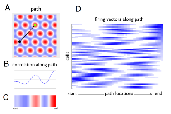
A. Overhead view of a square apparatus. The “Goal” is the green spot and current location the black spot. Colors are the correlation of each location with the goal firing vector. (Since this is a single module, lots of “false alarms”). B and C depict the correlations along a linear path. D depicts the firing of each cell in the module as the rat takes (or imagines) a linear path to the goal. Each cell is a horizontal stripe. The cells are arranged in rank order at the goal, so we see clear organization at the right.
 If we add two other modules, the correct path to the goal can extend greater distances, with fewer false alarms (right). This is also illustrated in the figure below where we see the firing vectors of the each of the three modules reach a peak, simultaneously, at the goal.

Three modules, coded by color. Although there is wavelike rhythmicity to in some groups, the three simultaneously reach high correlation at the goal.
This is the current state of the project. We have examined how a modular organization contributes to “linear look-ahead” both within a module and across modules. Most importantly, from our point of view, we have speculated on how the process of linear look ahead would contribute to solving complex navigational problems.
This is a sketch of how known brain circuits and parsimonious extensions could solve a complex cognitive problem. a complex cognitive problem. This is clearly a proposition, and far from truth. What we imagine might happen is, roughly, this. A rat sits at a location in a familiar environment, which elicits the current firing vector in grid cells. The rat remembers reward, and, via place cells, elicits the firing vector of grid cells at the reward location. Via a computational procedure the rat elicits a vector (direction and distance) that will lead from the current location to the reward location. Although the two locations must sit on the same visited space, the direct path can cross unvisited locations (figure at top). We have proposed a single mechanism, via linear look-ahead describing how this computation could be performed.
This is not the only possible solution. It should be noted, for example, that Erdem and Hasselmo have proposed a grid cell mechanism for linear look ahead that does not depend on organization of grid cells into discrete clusters. Nonetheless, we feel that the modular organization of grid cells has tremendous computational advantages that will continue to be recognized.
—-
* head-direction cells are neurons that fire when the rat’s nose is pointed in a particular direction. Similar to compass direction, but not locked to earth coordinates. They are recorded primarily in various parts of the hippocampal formation.
